AI for laypersons: Image recognition with nearest neighbors

Recap

In the last post we constructed our very first AI algorithm that was able to mimic the human decision whether a newly received email is unwanted “spam” or benign “ham”. We also established that the technical term “algorithm” actually only means a step-by-step description of how to translate input values into output values. For our spam detection algorithm we needed to find the database entry that has the maximum number of matching words between itself and the email that needs to be decided upon. Then we could just look up whether that database email was considered “spam” or “ham” and copy the same label for our output.

This algorithm was effective, but it only detected spam, so how could we possibly use it as a proxy for understanding all the different and complex AI systems out there? Well, in fact the nearest neighbor algorithm that we used as the basis for our spam detection AI, can be applied to a wide range of problems. In this post, I want to show you how it can be used for a problem that has nothing at all to do with spam detection, and that is image recognition.

A new task: Image recognition

Imagine you work in mail distribution center and have to find a way to sort letters by the handwritten zip codes on letter envelopes. This can and has for a long time been done by manual labor, but I imagine this is not anybody’s dream job. Instead, it would be nice if we could just pass the mail through a scanner, and then use a computer program to automatically extract the zip code from the scanner image. There are a whole lot of messy details in this process: The program needs to align the image, find the area on the envelope where the address is written, find the zip code within the address and separate the code into individual digits that it then needs to recognize. To keep things simple, we only focus on the last step: Recognizing a handwritten digit from a black and white scanner image.

Some examples may look like this (which are converted samples from an actual AI dataset called MNIST by Corinna Cortes, Christopher JC Burges, and Yann LeCun):

The “intelligent” decision we are looking for in this situation is to take one of these images and recognize which number is shown on it. For most of the above examples, this would be simple for a human, but there are also some instances that are a little more tricky:

• could be both a 1 or a 7.
• is somewhere between a 2 and a 3.
• might be confused for a 9 instead of an 8.

How computers see images

In order to automate this digit recognition task, we need to know how images are represented in a computer. You probably already know this, but to start from the beginning: Digital images are made up of small squares with uniform color and size, which are called pixels (short for “picture element”). To build up a whole image, these pixels are arranged in a regular grid of rows and columns. The images above all have 28 rows and 28 columns of pixels, which each can be either fully black or fully white. Let’s scale up one of these images to ten times its size to actually see the pixels.

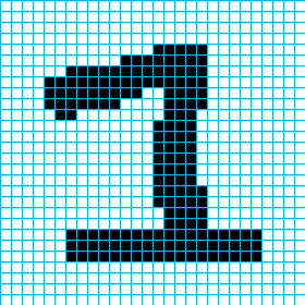
Now we are still talking about images in terms of colors and geometric terms instead of text or numbers that a computer can read and manipulate. One simple way of storing the above image in a machine-readable format is to create a text file and write a zero for each white pixel and a one for each black pixel, arranged in rows and columns and separated by spaces:

0 0 0 0 0 0 0 0 0 0 0 0 0 0 0 0 0 0 0 0 0 0 0 0 0 0 0 0
0 0 0 0 0 0 0 0 0 0 0 0 0 0 0 0 0 0 0 0 0 0 0 0 0 0 0 0
0 0 0 0 0 0 0 0 0 0 0 0 0 0 0 0 0 0 0 0 0 0 0 0 0 0 0 0
0 0 0 0 0 0 0 0 0 0 0 0 0 0 0 0 0 0 0 0 0 0 0 0 0 0 0 0
0 0 0 0 0 0 0 0 0 0 0 0 0 0 1 1 1 1 1 0 0 0 0 0 0 0 0 0
0 0 0 0 0 0 0 0 0 0 0 1 1 1 1 1 1 1 1 0 0 0 0 0 0 0 0 0
0 0 0 0 0 0 1 1 1 1 1 1 1 1 1 1 1 1 1 0 0 0 0 0 0 0 0 0
0 0 0 0 1 1 1 1 1 1 1 1 1 1 1 1 1 1 1 0 0 0 0 0 0 0 0 0
0 0 0 0 1 1 1 1 1 1 1 1 1 0 0 1 1 1 1 0 0 0 0 0 0 0 0 0
0 0 0 0 1 1 1 1 1 1 1 0 0 0 0 1 1 1 1 0 0 0 0 0 0 0 0 0
0 0 0 0 0 1 1 0 0 0 0 0 0 0 0 1 1 1 0 0 0 0 0 0 0 0 0 0
0 0 0 0 0 0 0 0 0 0 0 0 0 0 1 1 1 1 0 0 0 0 0 0 0 0 0 0
0 0 0 0 0 0 0 0 0 0 0 0 0 0 1 1 1 1 0 0 0 0 0 0 0 0 0 0
0 0 0 0 0 0 0 0 0 0 0 0 0 0 1 1 1 1 0 0 0 0 0 0 0 0 0 0
0 0 0 0 0 0 0 0 0 0 0 0 0 0 1 1 1 1 0 0 0 0 0 0 0 0 0 0
0 0 0 0 0 0 0 0 0 0 0 0 0 0 1 1 1 1 0 0 0 0 0 0 0 0 0 0
0 0 0 0 0 0 0 0 0 0 0 0 0 0 1 1 1 1 0 0 0 0 0 0 0 0 0 0
0 0 0 0 0 0 0 0 0 0 0 0 0 0 1 1 1 1 1 0 0 0 0 0 0 0 0 0
0 0 0 0 0 0 0 0 0 0 0 0 0 0 1 1 1 1 1 0 0 0 0 0 0 0 0 0
0 0 0 0 0 0 0 0 0 0 0 0 0 0 0 1 1 1 1 0 0 0 0 0 0 0 0 0
0 0 0 0 0 0 0 0 0 0 0 0 0 0 0 1 1 1 1 0 0 0 0 0 0 0 0 0
0 0 0 0 0 0 1 1 1 1 1 1 1 1 1 1 1 1 1 1 1 1 1 1 0 0 0 0
0 0 0 0 0 0 1 1 1 1 1 1 1 1 1 1 1 1 1 1 1 1 1 1 0 0 0 0
0 0 0 0 0 0 1 1 1 1 1 1 1 1 1 1 1 1 1 1 1 1 1 1 0 0 0 0
0 0 0 0 0 0 0 0 0 0 0 0 0 0 0 0 0 0 0 0 0 0 0 0 0 0 0 0
0 0 0 0 0 0 0 0 0 0 0 0 0 0 0 0 0 0 0 0 0 0 0 0 0 0 0 0
0 0 0 0 0 0 0 0 0 0 0 0 0 0 0 0 0 0 0 0 0 0 0 0 0 0 0 0
0 0 0 0 0 0 0 0 0 0 0 0 0 0 0 0 0 0 0 0 0 0 0 0 0 0 0 0

If you squint your eyes a little, you can even still see the picture, but now it is just a bunch of zeros and ones. This image format is called a Portable BitMap (PBM), and it can actually be read by open-source image editing tools like GIMP. If you want to, you can try it out by downloading the above image in PBM format.

The image formats that you are used to, like JPEG, PNG, or GIF, are much more complicated, but this is just because they are designed to save storage space. Whenever images are displayed on the screen or opened in an image editor, it is in some bitmap-like format.

Comparing images

Now that we know how represent images in a format that can be understood by a computer program, we can start thinking about how to adjust our nearest neighbor algorithm to cope with 28x28 pixel images of digits. First, let’s start by revisiting our spam detection algorithm:

Algorithm: Simple spam detector

Inputs:

• Database: list of labeled emails
• Query: unlabeled email that should be classified

Output:

• Label: the most fitting label for the query (either “spam” or “ham”)

Steps:

1. For all labeled emails in the database, calculate the number of matching words between that email and the query.
2. Find the database entry with the maximum number of matching words.
3. Output the label attached to this database entry.

There are a few things that we have to change to make this work with images. First, we have different inputs and outputs now. The Database is now a list of labeled images, where the label is the digit shown in the image. The Query is an unlabeled image that has to be recognized. And finally, the output is again a Label, but instead of only two options we now have to choose one of ten different labels that correspond to the ten digits from zero to nine.

Moving to the steps of the algorithm, the “number of matching words” is, of course, meaningless for images. However, we can match something else to find the “nearest neighbor” of an image: the pixels. We can count the number of matching pixels by moving through both pictures at the same time, starting at the top left, and moving in “reading” order from left to right and from top to bottom. Every time the pixels at corresponding positions of the two images match, we increase the count of matching pixels by one. When we reach the bottom right of the image, we will have the total number of matching pixels between both images.

To see that this works, let’s look at a small example with tiny 3x4 pixel images:

[Database entry 1:]

Label: 1

0 1 0
0 1 0
0 1 0
0 1 0


[Database entry 2:]

Label: 7

1 1 1
0 0 1
0 0 1
0 0 1


[Query image:]

1 1 1
0 0 1
0 1 0
1 0 0

We have two images in the database of the digits one and seven, both consisting of straight lines. The query image that we want to know about is another seven, but this time with a slanted lower line. Our AI now compares the query image to both database images to find the following:

Matches for entry 1:
0 1 0     1 1 1      x ✓ x
0 1 0  =  0 0 1  ->  ✓ x x
0 1 0     0 1 0      ✓ ✓ ✓
0 1 0     1 0 0      x x ✓

  Total number of matching pixels: 6


Matches for entry 2:
1 1 1     1 1 1      ✓ ✓ ✓
0 0 1  =  0 0 1  ->  ✓ ✓ ✓
0 0 1     0 1 0      ✓ x x
0 0 1     1 0 0      x ✓ x

  Total number of matching pixels: 8

Since database entry 2 has more matching pixels than database entry 1, our AI chooses to copy the label of entry 2 and correctly decides that the query image is a seven and not a one.

Now that we know that our idea works, the only thing that is left to do is to turn it into a new formal algorithm description:

Algorithm: Simple digit recognizer

Inputs:

• Database: list of labeled images
• Query: unlabeled image that should be recognized

Output:

• Label: the most fitting label for the query (0-9)

Steps:

1. For all labeled images in the database, calculate the number of matching pixels between that image and the query.
2. Find the database entry with the maximum number of matching pixels.
3. Output the label attached to this database entry.

As you can see, we only hat to change a few words. The resulting algorithm is still a nearest neighbor algorithm, it only needed to be adapted to find “neighbors” of images instead of emails.

Again, we have turned the human task “recognize the handwritten number in this image” into a set of instructions for a machine that is now able to mimic this human decision-making process and thus can be considered an AI. This also means that all implications that we have drawn for the spam detection algorithm are also valid for image recognition tasks. In particular, the “intelligence” of the algorithm still only comes from having good samples in the database that represent the set of possible inputs well. While the recognition of the slanted seven worked out fine in our simplified example, a database featuring larger images should definitely include both straight and slanted sevens, and possibly also sevens with an additional horizontal bar in the center. If it does not have enough of these examples, some sevens could be falsely recognized as ones or fours. In our mail distribution center setting, this could result in a delay in package delivery, as the package would initially end up in the wrong district, but real-world examples of image recognition systems based on too simple datasets can have far worse outcomes: If you have dark skin, you have a tenfold chance to be misidentified by state-of-the-art facial recognition software. This can lead to you not being able to pass through biometric passport validation at the airport or even a false identification as a criminal. A major source for this problem is likely the fact that the databases used to train these algorithms can have as much as 80% light-skinned persons. Of course these systems use more complicated algorithms than our nearest neighbor approach, but as in cooking, it is all about the ingredients. If you give a bunch of moldy vegetables to a Michelin star chef and to a home-cook, the chef might be able to produce a more tolerable looking dish than the home-cook, but you probably would not want to eat either one. This problem is endearingly called garbage in, garbage out. We will go into detail on this issue in one of the next posts of the series, but first we will take a little more time to explore the variety of possible application areas of the nearest neighbor algorithm.

Edits and Acknowledgements

Since it was first published, this article has undergone the following changes due to reader feedback:

• Added more detailed explanation of “garbage in, garbage out” (thanks to Annina)